
This week we learned about text analytics. Text analytics is one of the most powerful tools in analytics field because of its ability to analyze unstructured data. Unstructured data are things like text (from a video, document, voice recording, email, tweets, e.t.c.). Given that 80% of all the data is in unstructured form, there is a massive potential in the analysis of unstructured data. Most of the unstructured data by itself is not valuable. It is very hard to interpret the message by just looking at the text data. So, that is why text analytics comes handy as we can analyze these unstructured data in a systematic way – identify and categorize topics of discussion. We can find what’s the most used words, the topics that has been discussed, basically find out the sentiment of people or of a document.
“Text Analytics, also known as text mining, is the process of examining large collections of written resources to generate new information, and to transform the unstructured text into structured data for use in further analysis. Text mining identifies facts, relationships and assertions that would otherwise remain buried in the mass of textual big data”.
https://www.linguamatics.com/what-is-text-mining-nlp-machine-learning
“Natural language processing (or NLP) is a component of text mining that performs a special kind of linguistic analysis that essentially helps a machine”read” text. NLP uses a variety of methodologies to decipher the ambiguities in human language, including the following: automatic summarization, part-of-speech tagging, disambiguation, entity extraction and relations extraction, as well as disambiguation and natural language understanding and recognition”.
https://www.expertsystem.com/natural-language-processing-and-text-mining/
For text analytics, we follow the same analytical process that we have been doing throughout:
Staging > Structuring > Cleansing > Summarize > Visualize > Model
In text analytics there are 4 main recipes:
Sentiment analysis
Create word clouds
Generate topics
Extract people and places from text
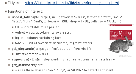
For this, in R, there is a package called tidytext and TM package for text mining. In addition, there a is a good free book Text Mining with R. For text mining, the functions of interests are unnest_tokens which parses the text into words and ngrams. ngrams would take the two words together, which words together occur in common. get_stopword that will actually pull out frequently used stop words and make a list of those stop words. For example and, a, the and common words that are just junk words. If we look at the frequency of them they would just skew our results. Stopwords eliminates junk from our analysis. It actually applies to the stop words, get_sentiments. We have couple different sentiment lexicons that are available to us, like NRC, Bing, AFINN
So for this week’s assignment, we were given the task to analyze Trump tweets. We went to Trump Twitter Archive which basically archives all Trump tweets that can be downloaded in a .csv file. I downloaded all the tweets (37,125) from May 2009 to August 18, 2019 for my analysis.
Load all the packages:
Tidyverse: our main package
Tidytext: Parsing and sentiment of text
Wordcloud and Wordcloud2: helps us visualize. Wordcloud2 actually makes nice little java scripts. Warning: when knitting documents in R notebook, sometimes those wordclouds don’t knit very well.
Lubridate: for dealing with dates
Stringr: dealing with strings
TM: a text mining package
Topicmodels: for topic models
CleanNLP or OpenNLP: for entity extraction.
“data.world”- host a number of nifty datasets that we can take advantage of for other text analysis scenarios.
library(dplyr)
library(tidyr)
library(purrr)
library(readr)
library(tidyverse)
library(lubridate)
library(tidytext)
library(wordcloud2)
library(ggplot2)
library(cleanNLP)
library(tm)
library(topicmodels)
library(magrittr)
However, given the massive number of Trump tweets, I decided to only analyze the tweets after Trump took over the Oval office in 2017. There were 9749 tweets remaining for us to analyze.
After staging, and structuring, we did word counts – produce a word frequency – using tidytext package and we used the function unnest_token, followed by anti join stop words which allows us to eliminate the stop words of the file. We also used filter string detect to filter out the numbers and used additional filter words to remove some of the words like https, realdonaldtrump, president, people, because these doesn’t add much value in our analysis. So I filtered those out and group them and I was able to create a frequency table by month and year. Then for sentiment analysis, I joined the frequency word that I created using bing lexicon sentiment analysis, and then created a bar chart.
#2.Sentiment Recipe
a.Create a word frequency data set by tokenize the tweet text, remove stop words, filter out numbers and junk, and finally summarize the words and arrange in descending order.
# --- parse and filter ------------------------------------------
tweet_freq <- tweets %>%
    unnest_tokens(word,text) %>%
    anti_join(stop_words) %>%
    filter(!str_detect(word,"^\\d")) %>%
    filter(!word %in% c("t.co","realdonaldtrump","https","http", "amp", "rt","twitter", "p.m", "president", "people", "trump"))
b. Join the word frequency data to the sentiments dataset, filter out positive negatives
c. Print the top 20 words and their sentiment
# --- join to Bing lexicon ----------------------------------------
tweet_sent <- tweet_freq %>%
    inner_join(get_sentiments("bing")) %>%
    filter(sentiment %in%
               c("positive","negative")) %>%
    select(mnth, word, sentiment) %>%
    group_by(word, sentiment) %>%
    summarise(n=n()) %>%
    arrange(sentiment,desc(n)) %>%
    ungroup() %>%
    top_n(20,n)
d. Create a bar chart of top 20 words, color by sentiment
# — make a chart —
tweet_sent %>%
    ggplot(aes(reorder(word, n),n, fill=sentiment)) +
    geom_col() +
    labs(y="Positive & Negative Sentiment",x= NULL) +
    coord_flip()
e. Create a second bar charts 20 words but use facet wrap to create two charts.
tweet_sent %>%
    ggplot(aes(reorder(word, n),n, fill=sentiment)) +
    geom_col() + facet_wrap(~sentiment, scales="free_y") +
    labs(y="contrib to sentiment",x= NULL) +
    coord_flip()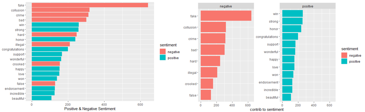
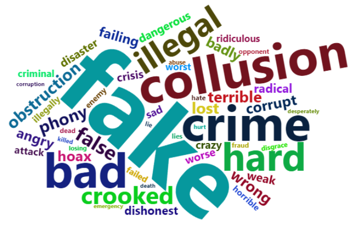
Generate Word Clouds
Next thing I did was word cloud using the same frequency table that I generated, and used the generate word cloud to function of the word cloud package, which helps us visualize easier.
tweet_sentTop100 <- tweet_freq %>%
    inner_join(get_sentiments("bing")) %>%
    filter(sentiment %in%
               c("positive","negative")) %>%
    select(mnth, word, sentiment) %>%
    group_by(word, sentiment) %>%
    summarise(n=n()) %>%
    arrange(sentiment,desc(n)) %>%
    ungroup() %>%
    top_n(100,n)

# --- make a chart ---
#a. Create a word cloud of the top 100 words used
tweet_sentTop100 %>%
    select(word,n) %>%
    wordcloud2()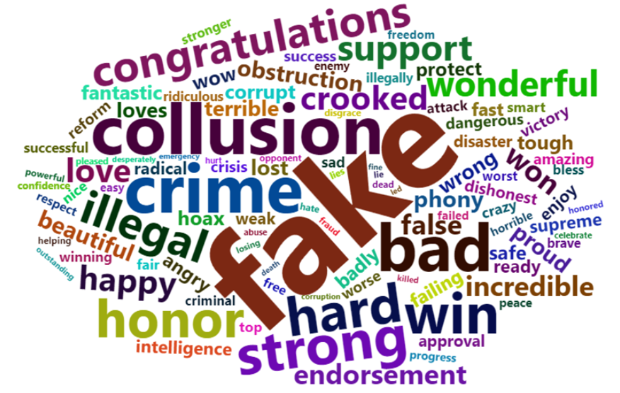

Next thing was to find out the topics that Trump was most concerned with. So for that we used topicmodel package that helps to generate topics. Using the same word frequency table, we create a term frequency metrics, and using the LDA method, we define value for K, basically the number assigned to K generates the number of topics that we want to generate in a dataset. For start, we used K=10, and then we visualize. It works like clustering technique that we previously learnt. So here’s the list of top 5 words identified that were used in the top 10 topics.
Identify Topics using Topicmodel package
Convert frequencies to a sparse matrix
## Convert frequencies to a sparse matrix

tweet_dtm <-
    tweet_freq %>%
    cast_dtm(document, word, n)
tweet_dtm
tweettopic_model  <- LDA(tweet_dtm, k = 10, control = list(seed = 1234))

tweet_topics <- tidy(tweettopic_model, matrix = "beta")
tweet_topics

tweet_top_terms <-
    tweet_topics %>%
    group_by(topic) %>%
    top_n(5, beta) %>%
    ungroup() %>%
    arrange(topic, -beta)

head(tweet_top_terms)

tweet_top_terms %>%
    mutate(term = reorder(term, beta)) %>%
    ggplot(aes(term, beta, fill = factor(topic))) +
    geom_col(show.legend = FALSE) +
    facet_wrap(~ topic, scales = "free") +
    coord_flip()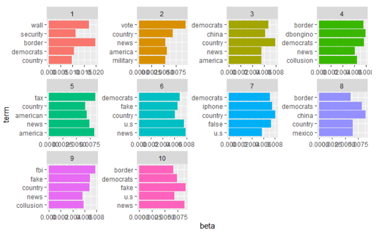
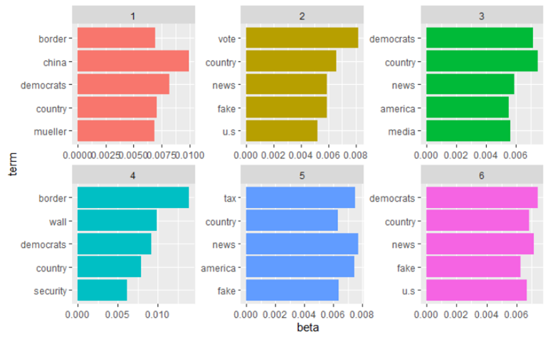
Instead of 10 topics, i wanted to narrow it down to 6 topics/issues that Trump used in his tweets on Twitter. From the bar chat below, we can categorize Trump tweets 6 topics: 1) China, 2) Vote, 3) Democrats, 4) Border and Wall 5) Tax, and 6) Fake News
This was a very fun practice exercise assignment, where we got to play with real social media texts and analyzed its sentiments and learned to summarize the top topics that person or people are talking/discussing about.
Reuse
Citation
@misc{shrestha2019,
  author = {Mohit Shrestha},
  title = {Text {Analytics}},
  date = {2019-08-19},
  url = {https://www.mohitshrestha.com.np/posts/2019-08-19-text-analytics},
  langid = {en}
}